Election Forensics: 2014 WI, FL, IL, MD Governor
Richard Charnin
Aug.13, 2015
Updated: Aug.17, 2015
Look inside the books: Reclaiming Science: The JFK Conspiracy … Matrix of Deceit: Forcing Pre-election and Exit Polls to Match Fraudulent Vote Counts
Compendium of Links to all of my posts
Cumulative Vote Share Spreadsheet Reference
An analysis of Exit Polls, True Votes and Cumulative Vote Shares indicates that the 2014 Governor elections in Wisconsin, Florida, Illinois and Maryland were likely stolen.
Although most voters believe that politicians are corrupt, many still cling to the myth that votes are accurately and fairly counted – and that election fraud is a conspiracy theory.
Many voters are still unaware that the unadjusted, pristine exit polls are routinely adjusted to match the recorded vote. The implicit assumption is that the recorded vote represents true voter intent.
Mathematical analysis of discrepancies between unadjusted presidential state and national exit polls versus recorded votes from 1988-2008 confirms systemic fraud to a 100% probability. For a suspicious election, mathematical analysis is a useful way to determine the likelihood of fraud.
Historical Analysis of Election Fraud
Pre-election polls
To set the context,Democrats do much better in Registered Voter (RV) polls than in the Likely Voter (LV) subsets. The reason is simple: voters considered unlikely to vote (mostly newly registered Democrats) are eliminated from the full RV sample. The RV polls are often close to the unadjusted exit polls and the True Vote. On the othr hand, final LV polls published on Election eve are excellent predictors of the bogus final recorded vote.
2012 Presidential Election- Final Forecast and True Vote
In each of the 1988, 1992, 2004 and 2008 presidential elections, in order for the pollsters to force the unadjusted exit polls to match the recorded vote, they needed to assume an impossible number of returning Republican voters. In the 1988-2008 presidential elections, the Democrats led the average recorded vote by 48-46%. But they led by 52-42% in the unadjusted state and national exit polls and the True Vote Model. The 8% margin discrepancy was far beyond the margin of error. But the discrepancy was not due to poor polling design, or exit poll respondents lying about their past vote, their current vote. They would have to lie in response to every one of dozens of questions.
Naysayers and media pundits want voters to believe that the exit polls are always wrong and must be “corrected” to conform to the recorded vote. But they never consider that the unadjusted exit polls are accurate and reflect true voter intent. To the pundits, election fraud is not a factor and the published exit polls accurately reflect voter intent. https://richardcharnin.wordpress.com/2011/11/13/1988-2008-unadjusted-state-exit-polls-statistical-reference/
But fraud is not limited to presidential elections. House, senate, governor and local elections have also been compromised by maliciously coded voting machines and voter disenfranchisement.
Who will argue with these points?
1- Unadjusted exit polls are hidden from the public.
2- Unadjusted exit polls are adjusted to match the recorded vote.
3- Voting machine software is proprietary, not open to public viewing
4- Auditing and hand-counting of votes are denied.
Exit polls
Since we cannot view unadjusted exit polls until years later (if at all), we are left with final, adjusted polls. The question “How did you vote in the last election” is no longer asked by the pollsters. An exhaustive analysis of 1988-2008 presidential election unadjusted state and national exit polls shows why the question is no longer asked: it gives an analyst the ability to check the number of returning voters from the prior election. The number provided in the adjusted polls has often proved to be impossible. There were more returning Bush voters in 1992, 2004 and 2008 than were alive. The 2004 election is a case in point. Simple arithmetic proves that it was stolen. It is a fact that…
1- Bush had 50.5 million recorded votes in 2000.
2- The 2004 National Exit Poll indicates that there were 52.6 million returning Bush 2000 voters. This is obviously impossible; the pollsters had to adjust the number of returning voters to match the 2004 recorded vote.
3- Of the 50.5 million Bush 2000 voters, approximately 2 million died before the 2004 election.
4- Approximately one million Bush 2000 voters did not return in 2004.
Therefore, an estimated 47.5 million Bush 2000 voters returned in 2004. Simple arithmetic shows there had to be at least 5 million (52.6-47.5) phantom Bush 2004 voters.
We are forced to analyze adjusted exit polls to look for anomalies. Party-ID is a demographic we can check in lieu of the past vote question. Of course, there is no way to check the Party-ID mix mathematically as we can with the past vote. But it is still useful to see if the percentage mix and corresponding vote shares are plausible based on voter registration and prior elections.
View the Party-ID sensitivity analysis for FL, IL, WI
https://docs.google.com/spreadsheets/d/1EGmR_gaXMGRWs4_iPYLNL7qsTDEkD5LMr-oTMJoOWQs/edit#gid=0
Florida 2014
True Vote Model
https://docs.google.com/spreadsheets/d/1SnErWihwCvq5puGw3sBF9E4jr585XV2NChqvxGObLAU/edit#gid=841488888
2014 True Vote
2-party Estimated
2010	True	Turnout	Votes	Mix	Crist	Scott

Sink	52.2%	93.0%	2.463	43.5%	92.5%	7.5%

Scott	47.8%	93.0%	2.255	39.9%	6.9%	93.1%

....................... True 	52.0%	48.0%

................... Recorded 49.4%	50.6%
Sensitivity Analysis
........Crist Share of Sink
Crist%..89.5% 92.5% 95.5%
Scott...Crist Total Share
9.9%....51.9% 53.2% 54.5%
6.9%....50.7% 52.0% 53.3%
3.9%....49.5% 50.8% 52.1%
........Crist Margin (000)
9.9%...211.69 359.47 507.25
6.9%....76.37 224.15 371.93
3.9%.. -58.96 88.824 236.61
In 2010, Sink (D) won the unadjusted exit poll by 50.8-45.4% (280,000 votes).There were 3150 respondents (2% margin of error). Of course, the poll was adjusted to match Scott’s 49.6-48.4% recorded 64,000 vote margin. It indicated that 47% of the voters were returning Obama voters and 47% McCain voters. But Obama won the Florida easily. Scott needed 67% of the other 6% who voted (new voters and others who voted for third parties in 2008). These adjustments are highly implausible.
To match the recorded vote, the pollsters assumed a 36D-36R-28I split with Scott winning Independents by 52-44%. In matching the unadjusted exit poll, Sink required a 38D-34R-28I split while winning Independents by 47-43%.
The 2014 election was virtually a carbon copy of 2010. Scott won by 48.2-47.1% (66,000 votes). Crist had 52% of the 2-party True Vote if Sink had the 52.2% share in the unadjusted 2010 exit poll. There were 500,000 more voters than in 2010. Historically, heavy voter turnout is good for the Democrats.
So how did Crist lose by 1%?
Crist did not lose. To match the recorded vote, the pollsters assumed an implausible Party-ID split: 31D- 35R- 34I. Assuming the true mix was 35D- 35R- 30I, Crist won by 181,000 votes (49.2-46.1%). According to the adjusted exit poll (assumed biased for Scott), Crist had 91% of Democrats; Scott had just 88% of Republicans. Crist won Independents by 46-44%. Crist shares were most likely higher.
Florida Exit Poll
(adjusted to match the recorded vote)……….True Vote
........Pct	Crist	Scott	Other...	Pct	Crist	Scott	Other

Dem.....31%	91.0%	6.00%	3.00%...	35.0%	92.0%	5.00%	3.00%

Rep.....35%	10.0%	88.0%	2.00%...	35.0%	10.0%	88.0%	2.00%

Other...33%	46.0%	44.0%	8.00%...	30.0%	46.0%	44.0%	10.0%

Total...99%	46.9%	47.2%	4.30%...	100.%	49.5%	45.8%	4.80%

Margin............17,044.............220,392
Sensitivity Analysis
................Crist Share of Dem
Dem Rep.....91.0% 92.0% 93.0%
................Crist Total share
32% 38%.....46.7% 47.0% 47.4%
35% 35%.....49.2% 49.5% 49.9%
38% 32%.....51.6% 52.0% 52.3%
................Crist Margin
32% 38%.....-1.8% -1.2% -0.5%
35% 35%......3.1% 3.8% 4.4%
38% 32%......7.9% 8.7% 9.4%
Illinois 2014
True Vote Model
https://docs.google.com/spreadsheets/d/1v6xm1XWdTYSEt5eXK1AegOY9iLx1ufseWVRzxQsz6N4/edit#gid=1727387709
Quinn won the True Vote assuming Obama’s 57% share and an equal 80% turnout of returning Obama and Romney voters.
2012 Votes Turnout.Vote. Pct.. Quinn. Rauner	Other

Obama...57.0%	1,686	1,349 38.5%	87.0%	12.0%	1%

Romney..42.0%	1,243	  994.. 28.4%	7.00%	93.0%	0%

Other....1.00%	00030	  24....0.7%	50.0%	49.0%	1%

DNV (new).......... 1,133. 32.4%	48.0%	48.0%	4%

Total...3,019	2,959 3,500..True 	1,799	1,642	59

................................51.4%	46.9%	1.7%

.......................Recorded 47.0%	51.9%	0.9%

...............................1,645	1,817	32

True Vote sensitivity analysis

Assumption: Quinn wins 48% of DNV/New voters
Quinn Quinn share of returning Obama voters
Share of 85.0% 87.0% 89.0%
Romney Quinn Vote Share
9%......51.2% 52.0% 52.7%
8%......50.9% 51.7% 52.5%
7%......50.6% 51.4% 52.2%
6%......50.3% 51.1% 51.9%
5%......50.1% 50.8% 51.6%
........Quinn Margin (000)
9%......143.0 196.9 250.9
8%......123.1 177.0 231.0
7%......103.2 157.2 211.1
6%.......83.3 137.3 191.2
5%.,.....63.4 117.4 171.4
Party-ID heavily favored the Democrats: 43D- 30R- 27I. Quinn had just 85% of Democrats and 29% of Independents. Assuming Quinn had 87% and 44%, respectively, he would have been a 50.8-45.6% winner.
Illinois Exit Poll
(adjusted to match recorded vote)……….True Vote
.........Pct	Quinn	Rauner	Other...Pct	Quinn	Rauner	Other

Dem.....43.0%	85.0%	13.0%	2.00%...43.0%	85.0%	12.0%	1.0%

Rep.....30.0%	5.00%	93.0%	2.00%...30.0%	5.00%	93.0%	2.0%

Other...26.0%	29.0%	64.0%	7.00%...27.0%	40.0%	52.0%	8.0%

Total...99.0%	45.6%	50.1%	3.30%...100.%	49.3%	47.1%	3.6%

Margin............164,643.............79,058
Sensitivity Analysis
............Quinn Share of Dem
Dem Rep.........85.0% 86.0% 87.0%
............Quinn Total share
42% 31%.....48.1% 48.5% 48.9%
43% 30%.....48.9% 49.3% 49.7%
44% 29%.....49.7% 50.1% 50.5%
............Quinn Margin
42% 31%....-0.3% 0.6% 1.4%
43% 30%.....1.3% 2.2% 3.0%
44% 29%.....2.9% 3.8% 4.7%
Wisconsin 2014
True Vote Model
https://docs.google.com/spreadsheets/d/1oAq0CJ1QSfy4JaNYpM_5esTafUdpt3ipgJU0Iz8RlD0/edit#gid=841488888
Burke won the True Vote, assuming that Barrett won the 2-party vote in 2012 by 53-47% and there was an equal returning voter turnout.
2-party	Estimated 	2014

2012....True	Turnout	Votes....	Mix	Burke	Walker

Barrett	53%     93%	1,207,636.......50.7%	92.7%	7.3%

Walker.	47%	93%	1,070,923.......45.0%	6.5%	93.5%

New..............101,962........4.3%	54.0%	46.0%

...........................True Vote	52.2%	47.8%

............................Recorded	47.1%	52.9%
Burke Share of Barrett
Share of.89.7% 92.7% 95.7%
Walker...Burke Share
9.5%.....52.1% 53.6% 55.1%
6.5%.....50.7% 52.3% 53.8%
3.5%.....49.4% 50.9% 52.4%
.........Burke Margin (000)
9.5%.....98.86 171.3 243.8
6.5%.....34.61 107.1 179.5
3.5%....-29.64 42.81 115.3
Party-ID was 36D- 37R- 27I, as opposed to 39D- 35R- 27I in prior elections. There was heavy voter turnout. Burke had just 43% of Independents. If the mix was actually 38D- 35R- 27I and Burke had 50% of independents, she would have been a 50.2-48.5% winner.
Wisconsin Exit Poll
(adjusted to match recorded vote)……….True Vote
........Pct	Burke	Walker	Other...Pct	Burke	Walker	Other

Dem.....36.0%	93.0%	6.00%	1.00%...38.0%	94.0%	5.00%	1.0%

Rep.....37.0%	4.00%	96.0%	0.00%...35.0%	4.00%	95.0%	1.0%

Other...27.0%	43.0%	54.0%	2.00%...27.0%	49.0%	49.0%	2.0%

Total...100.%	46.6%	52.3%	0.90%...100.%	50.4%	48.4%	1.3%

Margin............135,539..............46,936
Sensitivity Analysis
.............Burke Share of Dem
Dem Rep.....93.0% 94.0% 95.0%
.............Burke Total share
36% 37%.....48.2% 48.6% 48.9%
38% 35%.....50.0% 50.4% 50.7%
40% 33%.....51.8% 52.2% 52.6%
.............Burke Margin
36% 37%.....-2.4% -1.6% -0.9%
38% 35%......1.2% 2.0% 2.7%
40% 33%......4.8% 5.6% 6.4%
National Exit Poll (House)
The mix was 35D- 36R- 28I. The Republicans won by 52.0-45.8%. The Democrats had an implausibly low 42% of Independents. If the mix was 36D- 36R- 28I and the Democrats had 50% of the Independents, it would have been a virtual 49% tie.
Cumulative Vote Shares
It is well known fact that Democrats are the majority in highly populated urban locations; Republicans are heavily represented in rural areas. Highly populated precincts are mostly Democratic. But in scores of state elections there has been an increase in cumulative Republican vote shares in larger precincts. This anomaly has been confirmed by PhDs in Kansas and Vanderbilt University.
Consider the following changes from the 25% cumulative vote share to the final recorded share for five Governor elections (all but one competitive) and one senate election.
https://docs.google.com/spreadsheets/d/1dUBFrWmJxiopewHCUpHKbuTICmfcisJ9RXg48F-p1ec/edit#gid=0
-All 67 counties: Crist had 47.0% of 5.94 million votes
-12 Top counties: Crist had 52.0% of 3.67 million votes
-55 counties: Crist had 38.9% of 2.27 million votes
Top 12 counties, Crist’s 2-party share declined from 58.5% to 54.4%
Note: precinct data is not available for the 55 counties.
Wisconsin
https://docs.google.com/spreadsheet/ccc?key=0AjAk1JUWDMyRdEhqXzdlbUhZT1Vic3RSQmU2cUVkc3c#gid=12
-All 72 counties (2.59 million): Burke’s vote share declined from 49.1% to 46.6% (61.1 million)
-Top 15 counties (1.75 million votes): Burke’s vote share declined from 53.4% to 48.6% (76 mil. votes)
-Other 57 counties (0.84 million): Burke’s vote share increased from 40.8% to 42.6% (14.9 mil.)
-All 102 counties (3.63 million): Quinn’s vote share declined from 52.7% to 46.6% (227.7 million)
-Top 15 counties (2.79 million votes): Quinn’s vote share declined from 58.6% to 51.2% (205.8 million votes)
-87 counties (0.83 million): Quinn’s vote share declined from 33.1% to 30.4% (21.9 million)
Maryland
There is no exit poll for the MD governor election.
Hogan (R) defeated Brown (D) 53.88-46.12%
Hogan: 710,854, Brown 608,476 votes.
But note this anomaly:
Brown led by 53.9-44.5% in early and late votes (absentee and provisional ballots).
Hogan led election Day voting by 52.9-45.3%.
This also occurred in the 2000-2012 presidential elections. The Democrats always did much better in late voting. https://richardcharnin.wordpress.com/2013/01/09/election-fraud-2012-simple-algebra-of-early-election-day-and-late-recorded-votes/
MD	Early ElectDay	Absentee / Provisional

Brown	53.74%	45.31%	54.51%

......Early+Prov Elect Day  Total

Votes	390,340	1,342,837 1,733,177

Brown	53.91%	45.31%	47.20%

Hogan	44.46%	52.94%	51.00%
Hogan’s cumulative 2-party vote share increased from
50.3% at 25% of the total vote to 51.7% at 50% and 53.6% at 100%.
The 3.3% increase is a conservative estimate of the percentage of votes that may have been switched on Election Day given the 7% discrepancy between Election Day shares vs. Early and Late shares
CVS analysis for MD: https://docs.google.com/spreadsheets/d/17SpMcLyJ0607RyasTG4tRqrFmyDEKmEG45DKGGLZFmA/edit#gid=1626337891
2005 Special Ohio Congressional Election
Michael Collins has written about the GOP CVS trend in the 2005 Special Ohio congressional election and the 2012 primaries.
“Richard Charnin, posting as TruthIsAll, first noted the pattern with an analysis of the 2005 special election for a vacated seat for Ohio’s 2nd district, in the House of Representatives. The candidates were the liberal-populist Democrat Paul Hackett versus a right-wing Republican, Jean Schmidt. Charnin noticed that Schmidt’s votes and percentages increased substantially from the smallest to largest precincts in that district. This was a patently absurd pattern of vote accumulation since the liberal Hackett wins were in highly conservative counties that rarely voted for any Democrat.
Precincts with the most votes favored Schmidt at nearly 100%, with Hackett winning in only those with less than 200 votes counted. A review of precinct level results by Richard Charnin (TruthIsAll on Democratic Underground) reveals this interesting trend. This data is preliminary and more detail needs to be obtained from the Clermont Board of Elections. However, the trend observed for Clermont makes little sense on the face of it.
Hackett won 38 of 191 Clermont precincts with fewer than 187 votes, but lost ALL of the largest 54 precincts (those with more than 187 votes each). This is reflected in the following graph produced by Democratic Underground poster TruthIsAll, one of the first election fraud analysts to notice anomalies in Clermont County.
Hackett won 38 of 191 Clermont precincts but lost the 54 largest.
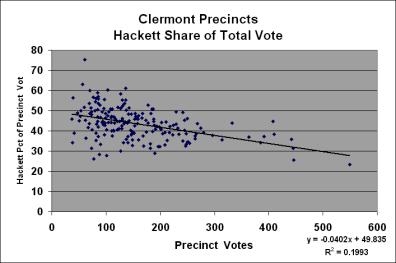
The following percentages help elaborate the graph above.
Hackett’s percentage by precinct group size:
46.9% in precincts under 100 votes
43.5% in precincts of 100-200 votes
39.6% in precincts of 200-300 votes
34.6% in precincts of 300 + votes
“Aside from the vote counting irregularities, other questions remain. Democrats typically do poorly in rural areas. A city-based attorney who supports the right to choose and refuses to support gay bashing legislation, who calls the President a “chicken hawk” and a “son of a bitch”, this candidate, Paul Hackett, carried the four most rural counties in District 2 by an average 59% to 41% margin. Yet this candidate failed in the more populous areas, where he would be expected to do better”.
These results raise interesting questions. Why does Hackett do much better in the smaller precincts? Are they more rural than the larger precincts? If so, does this not present a counterintuitive pattern, with the Democrat taking some of the conservative, less populated areas and the Republican winning all of the precincts in the most populated areas?
A question can be raised about the difference between turnout (the votes cast) and the actual size of the precinct, which may or may not be a reflection of votes cast. The following graph, also produced by TruthIsAll, answers the question. As he said while commenting on this data on 8/5/05: “The regression line has zero slope. Voters turned out at a fairly constant rate across precincts. So turnout wasn’t a factor in explaining why the Schmidt vote percentage increased as precinct size increased.”

Voter turnout in the larger precincts in Clermont County matches that in the overall 2nd District. Hackett sweeps rural, lower-income areas, while Schmidt takes those wealthier, more populous.
No Correlation between Precinct Registration and Voter Turnout
On the face of it, this is odd. The demographic blue-red maps for the 2004 election showed a positive correlation between population density and Democratic (Kerry) votes. Yet in the 2nd District of Ohio in 2005, the exact opposite was true.
Hackett dominated the least populated areas of the district, while Schmidt prevailed in the more populated areas. One observer said that Hackett performed as strongly as he did in rural District 2 because his handgun carry permit was publicized. This ignores the fact that the National Rifle Association endorsed Schmidt; it also ignores the generally prevailing positive attitude towards gun ownership in Southwest Ohio. This argument has one major problem. The NRA has one of the most disciplined political operations in the country. The members are consistent in following endorsements. The endorsement of Schmidt by NRA did not mean “think about voting for Schmidt” it meant “vote Schmidt.” Opposition from the NRA is a major impediment in rural areas.
2012 primaries
Consistent CVS anomalies in the 2012 GOP primaries favored Romney
Michael Collins wrote about it in a two-part article:
“Part I of this series suggested that there may well have been massive vote flipping for candidate Mitt Romney in the Republican primaries (Rigged Elections for Romney (10/22/12) The article and the initial research analysis were received broadly. In addition, highly motivated citizens across the country and a team of high school students contacted the authors for help replicating the research in their states. The researchers, Francois Choquet et al., point out that this can be done with their open source techniques.
The basic argument is straightforward. If you look at precinct level voting data arranged from the smallest to the largest precincts, you will see Romney’s gains increasing substantially as the cumulative vote increases. For example, Ohio and Wisconsin show this clearly as do eleven other states presented here. This extraordinary vote gain from smallest to largest precincts is so out of line, that the probability that this would happen by chance alone is often less than 1 out of a number represented by 1 preceded by 100 zeros and a decimal point, a value beneath the statistical package’s lower limits. As a result, the researchers termed the suspected vote flipping for Romney the “amazing anomaly.” (The Amazing Statistical Anomaly)
The research team’s observation of Romney gains based on precinct size is not unique. The anomaly was raised previously concerning the Republican presidential primaries on a political discussion forum.
Related links:
http://www.scoop.co.nz/stories/HL0508/S00186.htm
http://www.dailykos.com/story/2012/10/26/1150485/-Retired-NSA-Analyst-Proves-GOP-Is-Stealing-Elections#
Urban Legend:Implausible 2004 Bush vote shares in Urban counties.
http://www.richardcharnin.com/UrbanLegendLocation.htm
http://www.richardcharnin.com/LocationSizeKerryLandslide.htm
